Classifying Risky P2P Loans
Abstract
The prevalence of a global Peer-to-Peer (P2P) economy, coupled with the recent deregulation of financial markets, has lead to the widespread adoption of Artificial Intelligence driven by FinTech firms to manage risk when speculating on unsecured P2P debt obligations. After meticulously identifying ‘debt belonging to high-risk individuals’ by leveraging an ensemble of Machine Learning algorithms, these firms are able to find ideal trading opportunities.
While researching AI-driven portfolio management that favor risk-minimization strategies by unmasking subtle interactions amongst high dimensional features to identify prospective trades that exhibit modest ,low-risk gains, I was impressed that the overall portfolio: realized a modest return through a numerosity of individual gains; achieved an impressive Sharpe ratio stemming from infrequent losses and minimal portfolio volatility.
Project Overview
Objective
Build a binary classification model that predicts the “Charged Off” or “Fully Paid” Status of a loan by analyzing predominant characteristics which differentiate the two classes in order to engineer new features that may better enable our Machine Learning algorithms to reach efficacy in minimizing portfolio risk while observing better-than-average returns. Ultimately, the aim is to deploy this model to assist in placing trades on loans immediately after they are issued by Lending Club.
About P2P Lending
Peer-to-Peer (P2P) lending offers borrowers with bad credit to get the necessary funds to meet emergency deadlines. It might seem careless to lend even more money to people who have demonstrated an inability to repay loans in the past. However, by implementing Machine Learning algorithms to classify poor trade prospects, one can effectively minimize portfolio risk.
There is a large social component to P2P lending, for sociological factors (stigma of defaulting) often plays a greater role than financial metrics in determining an applicant’s creditworthiness. For example the “online friendships of borrowers act as signals of credit quality.” ( Lin et all, 2012)
The social benefit of providing finance for another individual has wonderful implications, and, while it is nice to engage in philanthropic activities, the motivating factor for underwriting speculating in p2p lending markets is financial gain, especially since the underlying debt is unsecured and investors are liable to defaults.
Project Setup
Import Libraries & Modules
from IPython.display import display
from IPython.core.display import HTML

import warnings
warnings.filterwarnings('ignore')

import os
if os.getcwd().split('/')[-1] == 'notebooks':
    os.chdir('../')
import pandas as pd
import numpy as np

import matplotlib
import matplotlib.pyplot as plt
import seaborn as sns

import pandas_profiling
from sklearn.model_selection import GridSearchCV
from sklearn.model_selection import StratifiedShuffleSplit
from sklearn.model_selection import train_test_split
from sklearn.pipeline import Pipeline
from sklearn.preprocessing import Imputer

from sklearn.dummy import DummyClassifier
from sklearn.ensemble import AdaBoostClassifier
from sklearn.ensemble import ExtraTreesClassifier
from sklearn.ensemble import GradientBoostingClassifier
from sklearn.ensemble import RandomForestClassifier
from sklearn.tree import DecisionTreeClassifier

# written by Gilles Louppe and distributed under the BSD 3 clause
from src.vn_datasci.blagging import BlaggingClassifier

from sklearn.metrics import accuracy_score
from sklearn.metrics import classification_report
from sklearn.metrics import fbeta_score
from sklearn.metrics import make_scorer
from sklearn.metrics import roc_auc_score
from sklearn.metrics import roc_curve
from sklearn.metrics import classification_report

# self-authored library that to facilatate ML classification and evaluation
from src.vn_datasci.skhelper import LearningModel, eval_db
Notebook Config
from IPython.display import display
from IPython.core.display import HTML

import warnings
warnings.filterwarnings('ignore')

import os
if os.getcwd().split('/')[-1] == 'notebooks':
    os.chdir('../')
%matplotlib inline
#%config figure_format='retina'
plt.rcParams.update({'figure.figsize': (10, 7)})

sns.set_context("notebook", font_scale=1.75, rc={"lines.linewidth": 1.25})
sns.set_style("darkgrid")
sns.set_palette("deep")

pd.options.display.width = 80
pd.options.display.max_columns = 50
pd.options.display.max_rows = 50
Data Preprocessing
Load Dataset
Data used for this project comes directly from Lending Club’s historical loan records (the full record contains more than 100 columns).
def load_dataset(path='data/raw/lc_historical.csv'):
    lc = pd.read_csv(path, index_col='id', memory_map=True, low_memory=False)
    lc.loan_status = pd.Categorical(lc.loan_status, categories=['Fully Paid', 'Charged Off'])
    return lc
dataset = load_dataset()
Exploration
Summary
Target: loan-status
Number of features: 18
Number of observations: 138196
Feature datatypes:
object: dti, bc_util, fico_range_low, percent_bc_gt_75, acc_open_past_24mths, annual_inc, recoveries, avg_cur_bal, loan_amnt
float64: revol_util, earliest_cr_line, purpose, emp_length, home_ownership, addr_state, issue_d, loan_status
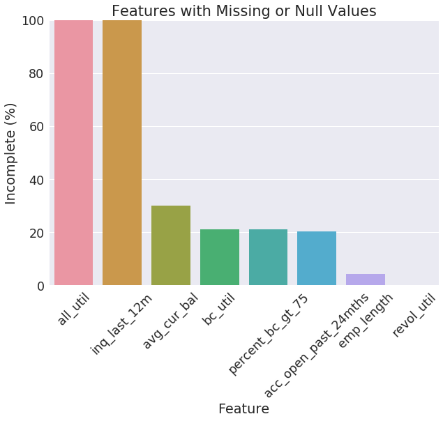
Features with ALL missing or null values:
inq_last_12m
all_util
Features with SOME missing or null values:
avg_cur_bal (30%)
bc_util (21%)
percent_bc_gt_75 (21%)
acc_open_past_24mths (20%)
emp_length (0.18%)
revol_util (0.08%)
Missing Data
Helper Functions
def calc_incomplete_stats(dataset):
    warnings.filterwarnings("ignore", 'This pattern has match groups')
    missing_data = pd.DataFrame(index=dataset.columns)
    missing_data['Null'] = dataset.isnull().sum()
    missing_data['NA_or_Missing'] = (
        dataset.apply(lambda col: (
            col.str.contains('(^$|n/a|^na$|^%$)', case=False).sum()))
        .fillna(0).astype(int))
    missing_data['Incomplete'] = (
        (missing_data.Null + missing_data.NA_or_Missing) / len(dataset))
    incomplete_stats = ((missing_data[(missing_data > 0).any(axis=1)])
                        .sort_values('Incomplete', ascending=False))
    return incomplete_stats

def display_incomplete_stats(incomplete_stats):
    stats = incomplete_stats.copy()
    df_incomplete = (
        stats.style
        .set_caption('Missing')
        .background_gradient(cmap=sns.light_palette("orange", as_cmap=True),
                             low=0, high=1, subset=['Null', 'NA_or_Missing'])
        .background_gradient(cmap=sns.light_palette("red", as_cmap=True),
                             low=0, high=.6, subset=['Incomplete'])
        .format({'Null': '{:,}', 'NA_or_Missing': '{:,}', 'Incomplete': '{:.1%}'}))
    display(df_incomplete)

def plot_incomplete_stats(incomplete_stats, ylim_range=(0, 100)):
    stats = incomplete_stats.copy()
    stats.Incomplete = stats.Incomplete * 100
    _ = sns.barplot(x=stats.index.tolist(), y=stats.Incomplete.tolist())
    for item in _.get_xticklabels():
        item.set_rotation(45)
    _.set(xlabel='Feature', ylabel='Incomplete (%)',
          title='Features with Missing or Null Values',
          ylim=ylim_range)
    plt.show()

def incomplete_data_report(dataset, display_stats=True, plot=True):
    incomplete_stats = calc_incomplete_stats(dataset)
    if display_stats:
        display_incomplete_stats(incomplete_stats)
    if plot:
        plot_incomplete_stats(incomplete_stats)


incomplete_stats = load_dataset().pipe(calc_incomplete_stats)
display(incomplete_stats)
| Null | NA_or_Missing | Incomplete | |
|---|---|---|---|
| all_util | 172745 | 0 | 1.000000 |
| inq_last_12m | 172745 | 0 | 1.000000 |
| avg_cur_bal | 51649 | 0 | 0.298990 |
| bc_util | 36407 | 0 | 0.210756 |
| percent_bc_gt_75 | 36346 | 0 | 0.210403 |
| acc_open_past_24mths | 35121 | 0 | 0.203311 |
| emp_length | 0 | 7507 | 0.043457 |
| revol_util | 144 | 0 | 0.000834 |
plot_incomplete_stats(incomplete_stats)
Data Munging
Cleaning
all_util, inq_last_12m
Drop features (all observations contain null/missing values)
revol_util
Remove the percent sign (%) from string
Convert to a float
earliest_cr_line, issue_d
Convert to datetime data type.
emp_length
Strip leading and trailing whitespace
Replace ‘< 1’ with ‘0.5’
Replace ‘10+’ with ‘10.5’
Fill null values with ‘-1.5’
Convert to float
def clean_data(lc):
    lc = lc.copy().dropna(axis=1, thresh=1)

    dt_features = ['earliest_cr_line', 'issue_d']
    lc[dt_features] = lc[dt_features].apply(
        lambda col: pd.to_datetime(col, format='%Y-%m-%d'), axis=0)

    cat_features =['purpose', 'home_ownership', 'addr_state']
    lc[cat_features] = lc[cat_features].apply(pd.Categorical, axis=0)

    lc.revol_util = (lc.revol_util
                     .str.extract('(\d+\.?\d?)', expand=False)
                     .astype('float'))

    lc.emp_length = (lc.emp_length
                     .str.extract('(< 1|10\+|\d+)', expand=False)
                     .replace('< 1', '0.5')
                     .replace('10+', '10.5')
                     .fillna('-1.5')
                     .astype('float'))
    return lc
dataset = load_dataset().pipe(clean_data)
Feature Engineering
New Features
loan_amnt_to_inc
the ratio of loan amount to annual income
earliest_cr_line_age
age of first credit line from when the loan was issued
avg_cur_bal_to_inc
the ratio of avg current balance to annual income
avg_cur_bal_to_loan_amnt
the ratio of avg current balance to loan amount
acc_open_past_24mths_groups
level of accounts opened in the last 2 yrs
def add_features(lc):
    # ratio of loan amount to annual income
    group_labels = ['low', 'avg', 'high']
    lc['loan_amnt_to_inc'] = (
        pd.cut((lc.loan_amnt / lc.annual_inc), 3, labels=['low', 'avg', 'high'])
        .cat.set_categories(['low', 'avg', 'high'], ordered=True))

    # age of first credit line from when the loan was issued
    lc['earliest_cr_line_age'] = (lc.issue_d - lc.earliest_cr_line).astype(int)

    # the ratio of avg current balance to annual income
    lc['avg_cur_bal_to_inc'] = lc.avg_cur_bal / lc.annual_inc

    # the ratio of avg current balance to loan amount
    lc['avg_cur_bal_to_loan_amnt'] = lc.avg_cur_bal / lc.loan_amnt

    # grouping level of accounts opened in the last 2 yrs
    lc['acc_open_past_24mths_groups'] = (
        pd.qcut(lc.acc_open_past_24mths, 3, labels=['low', 'avg', 'high'])
        .cat.add_categories(['unknown']).fillna('unknown')
        .cat.set_categories(['low', 'avg', 'high', 'unknown'], ordered=True))

    return lc
dataset = load_dataset().pipe(clean_data).pipe(add_features)
Drop Features
def drop_features(lc):
    target_leaks = ['recoveries', 'issue_d']
    other_features = ['earliest_cr_line', 'acc_open_past_24mths', 'addr_state']
    to_drop = target_leaks + other_features
    return lc.drop(to_drop, axis=1)
dataset = load_dataset().pipe(clean_data).pipe(add_features).pipe(drop_features)
Load & Prepare Function
def load_and_preprocess_data():
    return (load_dataset()
            .pipe(clean_data)
            .pipe(add_features)
            .pipe(drop_features))
Exploratory Data Analysis (EDA)
Helper Functions
def plot_factor_pct(dataset, feature):
    if feature not in dataset.columns:
        return
    y = dataset[feature]
    factor_counts = y.value_counts()
    x_vals = factor_counts.index.tolist()
    y_vals = ((factor_counts.values/factor_counts.values.sum())*100).round(2)
    sns.barplot(y=x_vals, x=y_vals);

def plot_pct_charged_off(lc, feature):
    lc_counts = lc[feature].value_counts()
    charged_off = lc[lc.loan_status=='Charged Off']
    charged_off_counts = charged_off[feature].value_counts()
    charged_off_ratio = ((charged_off_counts / lc_counts * 100)
                         .round(2).sort_values(ascending=False))

    x_vals = charged_off_ratio.index.tolist()
    y_vals = charged_off_ratio
    sns.barplot(y=x_vals, x=y_vals);
Overview
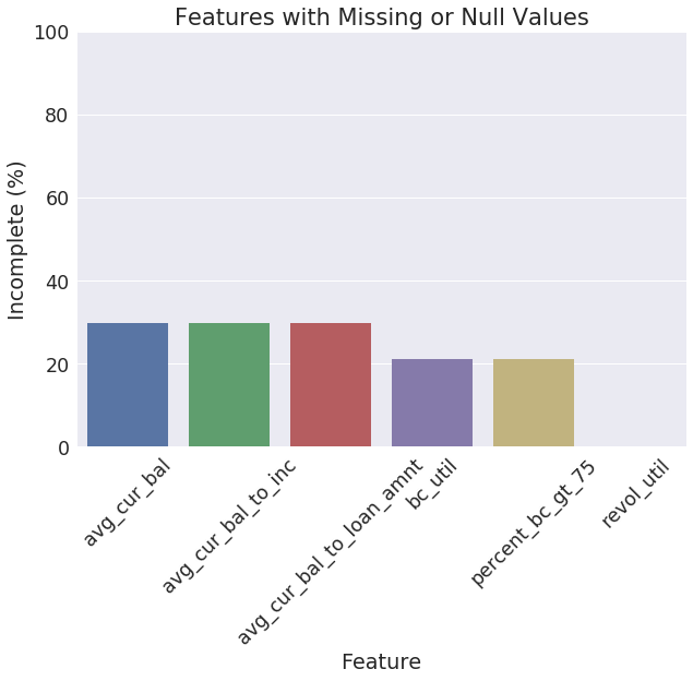
Missing Data
processed_dataset = load_and_preprocess_data()
incomplete_stats = calc_incomplete_stats(processed_dataset)
display(incomplete_stats)
| Null | NA_or_Missing | Incomplete | |
|---|---|---|---|
| avg_cur_bal | 51649 | 0 | 0.298990 |
| avg_cur_bal_to_inc | 51649 | 0 | 0.298990 |
| avg_cur_bal_to_loan_amnt | 51649 | 0 | 0.298990 |
| bc_util | 36407 | 0 | 0.210756 |
| percent_bc_gt_75 | 36346 | 0 | 0.210403 |
| revol_util | 144 | 0 | 0.000834 |
plot_incomplete_stats(incomplete_stats)
Summary Statistics
HTML(processed_dataset.pipe(pandas_profiling.ProfileReport).html)
Overview
Dataset info
| Number of variables | 18 |
|---|---|
| Number of observations | 172745 |
| Total Missing (%) | 7.3% |
| Total size in memory | 18.0 MiB |
| Average record size in memory | 109.0 B |
Variables types
| Numeric | 13 |
|---|---|
| Categorical | 5 |
| Date | 0 |
| Text (Unique) | 0 |
| Rejected | 0 |
Warnings
annual_incis highly skewed (γ1 = 35.012)avg_cur_balhas 51649 / 29.9% missing values Missingavg_cur_bal_to_inchas 51649 / 29.9% missing values Missingavg_cur_bal_to_loan_amnthas 51649 / 29.9% missing values Missingbc_utilhas 36407 / 21.1% missing values Missingpercent_bc_gt_75has 21592 / 12.5% zerospercent_bc_gt_75has 36346 / 21.0% missing values Missing
Variables
acc_open_past_24mths_groups
Categorical
| Distinct count | 4 |
|---|---|
| Unique (%) | 0.0% |
| Missing (%) | 0.0% |
| Missing (n) | 0 |
| avg | |
|---|---|
| low | |
| unknown |
| Value | Count | Frequency (%) | |
| avg | 59367 | 34.4% | |
| low | 46567 | 27.0% | |
| unknown | 35121 | 20.3% | |
| high | 31690 | 18.3% |
annual_inc
Numeric
| Distinct count | 14645 |
|---|---|
| Unique (%) | 8.5% |
| Missing (%) | 0.0% |
| Missing (n) | 0 |
| Infinite (%) | 0.0% |
| Infinite (n) | 0 |
| Mean | 69396 |
|---|---|
| Minimum | 4000 |
| Maximum | 7141800 |
| Zeros (%) | 0.0% |

Quantile statistics
| Minimum | 4000 |
|---|---|
| 5-th percentile | 25500 |
| Q1 | 42000 |
| Median | 60000 |
| Q3 | 84450 |
| 95-th percentile | 141000 |
| Maximum | 7141800 |
| Range | 7137800 |
| Interquartile range | 42450 |
Descriptive statistics
| Standard deviation | 55278 |
|---|---|
| Coef of variation | 0.79657 |
| Kurtosis | 3573.1 |
| Mean | 69396 |
| MAD | 29465 |
| Skewness | 35.012 |
| Sum | 11988000000 |
| Variance | 3055700000 |
| Memory size | 1.3 MiB |

| Value | Count | Frequency (%) | |
| 60000.0 | 6513 | 3.8% | |
| 50000.0 | 6008 | 3.5% | |
| 40000.0 | 5135 | 3.0% | |
| 45000.0 | 4651 | 2.7% | |
| 65000.0 | 4538 | 2.6% | |
| 70000.0 | 4224 | 2.4% | |
| 75000.0 | 4035 | 2.3% | |
| 55000.0 | 3972 | 2.3% | |
| 80000.0 | 3971 | 2.3% | |
| 30000.0 | 3512 | 2.0% | |
| Other values (14635) | 126186 | 73.0% |
Minimum 5 values
| Value | Count | Frequency (%) | |
| 4000.0 | 1 | 0.0% | |
| 4080.0 | 1 | 0.0% | |
| 4200.0 | 2 | 0.0% | |
| 4800.0 | 3 | 0.0% | |
| 4888.0 | 1 | 0.0% |
Maximum 5 values
| Value | Count | Frequency (%) | |
| 2039784.0 | 1 | 0.0% | |
| 5000000.0 | 1 | 0.0% | |
| 6000000.0 | 1 | 0.0% | |
| 6100000.0 | 1 | 0.0% | |
| 7141778.0 | 1 | 0.0% |
avg_cur_bal
Numeric
| Distinct count | 36973 |
|---|---|
| Unique (%) | 30.5% |
| Missing (%) | 29.9% |
| Missing (n) | 51649 |
| Infinite (%) | 0.0% |
| Infinite (n) | 0 |
| Mean | 12920 |
|---|---|
| Minimum | 0 |
| Maximum | 958080 |
| Zeros (%) | 0.0% |

Quantile statistics
| Minimum | 0 |
|---|---|
| 5-th percentile | 1041 |
| Q1 | 2692 |
| Median | 6441 |
| Q3 | 18246 |
| 95-th percentile | 42192 |
| Maximum | 958080 |
| Range | 958080 |
| Interquartile range | 15554 |
Descriptive statistics
| Standard deviation | 16414 |
|---|---|
| Coef of variation | 1.2704 |
| Kurtosis | 170.13 |
| Mean | 12920 |
| MAD | 11074 |
| Skewness | 6.0427 |
| Sum | 1564600000 |
| Variance | 269430000 |
| Memory size | 1.3 MiB |

| Value | Count | Frequency (%) | |
| 1250.0 | 28 | 0.0% | |
| 2352.0 | 27 | 0.0% | |
| 2120.0 | 27 | 0.0% | |
| 2589.0 | 27 | 0.0% | |
| 0.0 | 26 | 0.0% | |
| 1583.0 | 26 | 0.0% | |
| 1336.0 | 26 | 0.0% | |
| 2587.0 | 26 | 0.0% | |
| 1971.0 | 26 | 0.0% | |
| 1724.0 | 26 | 0.0% | |
| Other values (36962) | 120831 | 69.9% | |
| (Missing) | 51649 | 29.9% |
Minimum 5 values
| Value | Count | Frequency (%) | |
| 0.0 | 26 | 0.0% | |
| 1.0 | 1 | 0.0% | |
| 2.0 | 1 | 0.0% | |
| 3.0 | 1 | 0.0% | |
| 4.0 | 2 | 0.0% |
Maximum 5 values
| Value | Count | Frequency (%) | |
| 383983.0 | 1 | 0.0% | |
| 477255.0 | 1 | 0.0% | |
| 502002.0 | 1 | 0.0% | |
| 800008.0 | 1 | 0.0% | |
| 958084.0 | 1 | 0.0% |
avg_cur_bal_to_inc
Numeric
| Distinct count | 103048 |
|---|---|
| Unique (%) | 85.1% |
| Missing (%) | 29.9% |
| Missing (n) | 51649 |
| Infinite (%) | 0.0% |
| Infinite (n) | 0 |
| Mean | 0.18212 |
|---|---|
| Minimum | 0 |
| Maximum | 6.3872 |
| Zeros (%) | 0.0% |

Quantile statistics
| Minimum | 0 |
|---|---|
| 5-th percentile | 0.020754 |
| Q1 | 0.050874 |
| Median | 0.11024 |
| Q3 | 0.2552 |
| 95-th percentile | 0.55037 |
| Maximum | 6.3872 |
| Range | 6.3872 |
| Interquartile range | 0.20432 |
Descriptive statistics
| Standard deviation | 0.19319 |
|---|---|
| Coef of variation | 1.0608 |
| Kurtosis | 21.742 |
| Mean | 0.18212 |
| MAD | 0.13916 |
| Skewness | 2.8321 |
| Sum | 22054 |
| Variance | 0.037321 |
| Memory size | 1.3 MiB |

| Value | Count | Frequency (%) | |
| 0.0 | 26 | 0.0% | |
| 0.041 | 21 | 0.0% | |
| 0.045 | 20 | 0.0% | |
| 0.044 | 19 | 0.0% | |
| 0.075 | 19 | 0.0% | |
| 0.05 | 18 | 0.0% | |
| 0.054 | 17 | 0.0% | |
| 0.042 | 17 | 0.0% | |
| 0.034 | 17 | 0.0% | |
| 0.06 | 17 | 0.0% | |
| Other values (103037) | 120905 | 70.0% | |
| (Missing) | 51649 | 29.9% |
Minimum 5 values
| Value | Count | Frequency (%) | |
| 0.0 | 26 | 0.0% | |
| 2.77777777778e-05 | 1 | 0.0% | |
| 4.44444444444e-05 | 1 | 0.0% | |
| 4.7619047619e-05 | 1 | 0.0% | |
| 0.000120481927711 | 1 | 0.0% |
Maximum 5 values
| Value | Count | Frequency (%) | |
| 3.19985833333 | 1 | 0.0% | |
| 3.36695 | 1 | 0.0% | |
| 3.5543 | 1 | 0.0% | |
| 3.68520833333 | 1 | 0.0% | |
| 6.38722666667 | 1 | 0.0% |
avg_cur_bal_to_loan_amnt
Numeric
| Distinct count | 95901 |
|---|---|
| Unique (%) | 79.2% |
| Missing (%) | 29.9% |
| Missing (n) | 51649 |
| Infinite (%) | 0.0% |
| Infinite (n) | 0 |
| Mean | 1.374 |
|---|---|
| Minimum | 0 |
| Maximum | 172.55 |
| Zeros (%) | 0.0% |
Quantile statistics
| Minimum | 0 |
|---|---|
| 5-th percentile | 0.10397 |
| Q1 | 0.2542 |
| Median | 0.62682 |
| Q3 | 1.5551 |
| 95-th percentile | 4.7668 |
| Maximum | 172.55 |
| Range | 172.55 |
| Interquartile range | 1.3009 |
Descriptive statistics
| Standard deviation | 2.574 |
|---|---|
| Coef of variation | 1.8734 |
| Kurtosis | 337.31 |
| Mean | 1.374 |
| MAD | 1.2728 |
| Skewness | 11.39 |
| Sum | 166380 |
| Variance | 6.6256 |
| Memory size | 1.3 MiB |

| Value | Count | Frequency (%) | |
| 0.0 | 26 | 0.0% | |
| 0.28 | 22 | 0.0% | |
| 0.16 | 21 | 0.0% | |
| 0.18 | 18 | 0.0% | |
| 0.196 | 18 | 0.0% | |
| 0.32 | 17 | 0.0% | |
| 0.15 | 17 | 0.0% | |
| 0.3 | 16 | 0.0% | |
| 0.14 | 16 | 0.0% | |
| 0.384 | 16 | 0.0% | |
| Other values (95890) | 120909 | 70.0% | |
| (Missing) | 51649 | 29.9% |
Minimum 5 values
| Value | Count | Frequency (%) | |
| 0.0 | 26 | 0.0% | |
| 0.000129032258065 | 1 | 0.0% | |
| 0.000182648401826 | 1 | 0.0% | |
| 0.000347826086957 | 1 | 0.0% | |
| 0.000444444444444 | 1 | 0.0% |
Maximum 5 values
| Value | Count | Frequency (%) | |
| 88.445 | 1 | 0.0% | |
| 90.194 | 1 | 0.0% | |
| 101.27 | 1 | 0.0% | |
| 108.851 | 1 | 0.0% | |
| 172.548 | 1 | 0.0% |
bc_util
Numeric
| Distinct count | 1178 |
|---|---|
| Unique (%) | 0.9% |
| Missing (%) | 21.1% |
| Missing (n) | 36407 |
| Infinite (%) | 0.0% |
| Infinite (n) | 0 |
| Mean | 66.058 |
|---|---|
| Minimum | 0 |
| Maximum | 339.6 |
| Zeros (%) | 0.7% |

Quantile statistics
| Minimum | 0 |
|---|---|
| 5-th percentile | 14.4 |
| Q1 | 48.2 |
| Median | 71.3 |
| Q3 | 88.5 |
| 95-th percentile | 98.4 |
| Maximum | 339.6 |
| Range | 339.6 |
| Interquartile range | 40.3 |
Descriptive statistics
| Standard deviation | 26.359 |
|---|---|
| Coef of variation | 0.39902 |
| Kurtosis | -0.37079 |
| Mean | 66.058 |
| MAD | 21.95 |
| Skewness | -0.65476 |
| Sum | 9006300 |
| Variance | 694.79 |
| Memory size | 1.3 MiB |

| Value | Count | Frequency (%) | |
| 0.0 | 1153 | 0.7% | |
| 98.2 | 350 | 0.2% | |
| 97.4 | 349 | 0.2% | |
| 97.9 | 347 | 0.2% | |
| 98.6 | 340 | 0.2% | |
| 96.8 | 337 | 0.2% | |
| 98.3 | 332 | 0.2% | |
| 97.5 | 331 | 0.2% | |
| 97.3 | 329 | 0.2% | |
| 97.7 | 325 | 0.2% | |
| Other values (1167) | 132145 | 76.5% | |
| (Missing) | 36407 | 21.1% |
Minimum 5 values
| Value | Count | Frequency (%) | |
| 0.0 | 1153 | 0.7% | |
| 0.1 | 81 | 0.0% | |
| 0.2 | 67 | 0.0% | |
| 0.3 | 61 | 0.0% | |
| 0.4 | 53 | 0.0% |
Maximum 5 values
| Value | Count | Frequency (%) | |
| 165.7 | 1 | 0.0% | |
| 173.2 | 1 | 0.0% | |
| 182.5 | 1 | 0.0% | |
| 187.9 | 1 | 0.0% | |
| 339.6 | 1 | 0.0% |
dti
Numeric
| Distinct count | 3499 |
|---|---|
| Unique (%) | 2.0% |
| Missing (%) | 0.0% |
| Missing (n) | 0 |
| Infinite (%) | 0.0% |
| Infinite (n) | 0 |
| Mean | 16.08 |
|---|---|
| Minimum | 0 |
| Maximum | 34.99 |
| Zeros (%) | 0.1% |

Quantile statistics
| Minimum | 0 |
|---|---|
| 5-th percentile | 4.08 |
| Q1 | 10.34 |
| Median | 15.74 |
| Q3 | 21.52 |
| 95-th percentile | 29.28 |
| Maximum | 34.99 |
| Range | 34.99 |
| Interquartile range | 11.18 |
Descriptive statistics
| Standard deviation | 7.6032 |
|---|---|
| Coef of variation | 0.47285 |
| Kurtosis | -0.60719 |
| Mean | 16.08 |
| MAD | 6.2649 |
| Skewness | 0.17839 |
| Sum | 2777700 |
| Variance | 57.809 |
| Memory size | 1.3 MiB |

| Value | Count | Frequency (%) | |
| 0.0 | 220 | 0.1% | |
| 14.4 | 186 | 0.1% | |
| 16.8 | 153 | 0.1% | |
| 12.0 | 152 | 0.1% | |
| 18.0 | 143 | 0.1% | |
| 19.2 | 139 | 0.1% | |
| 20.4 | 138 | 0.1% | |
| 15.6 | 137 | 0.1% | |
| 13.2 | 137 | 0.1% | |
| 21.6 | 130 | 0.1% | |
| Other values (3489) | 171210 | 99.1% |
Minimum 5 values
| Value | Count | Frequency (%) | |
| 0.0 | 220 | 0.1% | |
| 0.01 | 6 | 0.0% | |
| 0.02 | 6 | 0.0% | |
| 0.03 | 3 | 0.0% | |
| 0.04 | 4 | 0.0% |
Maximum 5 values
| Value | Count | Frequency (%) | |
| 34.95 | 11 | 0.0% | |
| 34.96 | 9 | 0.0% | |
| 34.97 | 7 | 0.0% | |
| 34.98 | 13 | 0.0% | |
| 34.99 | 9 | 0.0% |
earliest_cr_line_age
Numeric
| Distinct count | 2173 |
|---|---|
| Unique (%) | 1.3% |
| Missing (%) | 0.0% |
| Missing (n) | 0 |
| Infinite (%) | 0.0% |
| Infinite (n) | 0 |
| Mean | 4.7171e+17 |
|---|---|
| Minimum | 94608000000000000 |
| Maximum | 2064268800000000000 |
| Zeros (%) | 0.0% |

Quantile statistics
| Minimum | 94608000000000000 |
|---|---|
| 5-th percentile | 1.7876e+17 |
| Q1 | 3.2072e+17 |
| Median | 4.2863e+17 |
| Q3 | 5.813e+17 |
| 95-th percentile | 9.0729e+17 |
| Maximum | 2064268800000000000 |
| Range | 1969660800000000000 |
| Interquartile range | 2.6058e+17 |
Descriptive statistics
| Standard deviation | 2.2491e+17 |
|---|---|
| Coef of variation | 0.4768 |
| Kurtosis | 1.7574 |
| Mean | 4.7171e+17 |
| MAD | 1.7187e+17 |
| Skewness | 1.1264 |
| Sum | 6909064824910512128 |
| Variance | 5.0585e+34 |
| Memory size | 1.3 MiB |

| Value | Count | Frequency (%) | |
| 378691200000000000 | 1085 | 0.6% | |
| 347155200000000000 | 866 | 0.5% | |
| 373420800000000000 | 846 | 0.5% | |
| 441849600000000000 | 821 | 0.5% | |
| 410227200000000000 | 782 | 0.5% | |
| 383961600000000000 | 749 | 0.4% | |
| 473385600000000000 | 737 | 0.4% | |
| 386640000000000000 | 732 | 0.4% | |
| 381369600000000000 | 706 | 0.4% | |
| 504921600000000000 | 694 | 0.4% | |
| Other values (2163) | 164727 | 95.4% |
Minimum 5 values
| Value | Count | Frequency (%) | |
| 94608000000000000 | 4 | 0.0% | |
| 94694400000000000 | 17 | 0.0% | |
| 97113600000000000 | 5 | 0.0% | |
| 97200000000000000 | 7 | 0.0% | |
| 97286400000000000 | 49 | 0.0% |
Maximum 5 values
| Value | Count | Frequency (%) | |
| 1838246400000000000 | 1 | 0.0% | |
| 1888185600000000000 | 1 | 0.0% | |
| 1930435200000000000 | 1 | 0.0% | |
| 1972252800000000000 | 1 | 0.0% | |
| 2064268800000000000 | 1 | 0.0% |
emp_length
Numeric
| Distinct count | 12 |
|---|---|
| Unique (%) | 0.0% |
| Missing (%) | 0.0% |
| Missing (n) | 0 |
| Infinite (%) | 0.0% |
| Infinite (n) | 0 |
| Mean | 5.5865 |
|---|---|
| Minimum | -1.5 |
| Maximum | 10.5 |
| Zeros (%) | 0.0% |

Quantile statistics
| Minimum | -1.5 |
|---|---|
| 5-th percentile | 0.5 |
| Q1 | 2 |
| Median | 5 |
| Q3 | 10.5 |
| 95-th percentile | 10.5 |
| Maximum | 10.5 |
| Range | 12 |
| Interquartile range | 8.5 |
Descriptive statistics
| Standard deviation | 3.9298 |
|---|---|
| Coef of variation | 0.70344 |
| Kurtosis | -1.37 |
| Mean | 5.5865 |
| MAD | 3.4876 |
| Skewness | -0.046929 |
| Sum | 965040 |
| Variance | 15.443 |
| Memory size | 1.3 MiB |

| Value | Count | Frequency (%) | |
| 10.5 | 49479 | 28.6% | |
| 2.0 | 16294 | 9.4% | |
| 0.5 | 14318 | 8.3% | |
| 3.0 | 14219 | 8.2% | |
| 5.0 | 13433 | 7.8% | |
| 1.0 | 11862 | 6.9% | |
| 4.0 | 11162 | 6.5% | |
| 6.0 | 10784 | 6.2% | |
| 7.0 | 9689 | 5.6% | |
| 8.0 | 7819 | 4.5% | |
| Other values (2) | 13686 | 7.9% |
Minimum 5 values
| Value | Count | Frequency (%) | |
| -1.5 | 7507 | 4.3% | |
| 0.5 | 14318 | 8.3% | |
| 1.0 | 11862 | 6.9% | |
| 2.0 | 16294 | 9.4% | |
| 3.0 | 14219 | 8.2% |
Maximum 5 values
| Value | Count | Frequency (%) | |
| 6.0 | 10784 | 6.2% | |
| 7.0 | 9689 | 5.6% | |
| 8.0 | 7819 | 4.5% | |
| 9.0 | 6179 | 3.6% | |
| 10.5 | 49479 | 28.6% |
fico_range_low
Numeric
| Distinct count | 40 |
|---|---|
| Unique (%) | 0.0% |
| Missing (%) | 0.0% |
| Missing (n) | 0 |
| Infinite (%) | 0.0% |
| Infinite (n) | 0 |
| Mean | 699.97 |
|---|---|
| Minimum | 625 |
| Maximum | 845 |
| Zeros (%) | 0.0% |

Quantile statistics
| Minimum | 625 |
|---|---|
| 5-th percentile | 660 |
| Q1 | 675 |
| Median | 695 |
| Q3 | 715 |
| 95-th percentile | 765 |
| Maximum | 845 |
| Range | 220 |
| Interquartile range | 40 |
Descriptive statistics
| Standard deviation | 32.182 |
|---|---|
| Coef of variation | 0.045977 |
| Kurtosis | 1.1327 |
| Mean | 699.97 |
| MAD | 25.082 |
| Skewness | 1.1394 |
| Sum | 120920000 |
| Variance | 1035.7 |
| Memory size | 1.3 MiB |

| Value | Count | Frequency (%) | |
| 680.0 | 13161 | 7.6% | |
| 670.0 | 12875 | 7.5% | |
| 675.0 | 12564 | 7.3% | |
| 690.0 | 12290 | 7.1% | |
| 685.0 | 12278 | 7.1% | |
| 665.0 | 11832 | 6.8% | |
| 695.0 | 11174 | 6.5% | |
| 660.0 | 10712 | 6.2% | |
| 700.0 | 10333 | 6.0% | |
| 705.0 | 9309 | 5.4% | |
| Other values (30) | 56217 | 32.5% |
Minimum 5 values
| Value | Count | Frequency (%) | |
| 625.0 | 1 | 0.0% | |
| 630.0 | 1 | 0.0% | |
| 660.0 | 10712 | 6.2% | |
| 665.0 | 11832 | 6.8% | |
| 670.0 | 12875 | 7.5% |
Maximum 5 values
| Value | Count | Frequency (%) | |
| 825.0 | 115 | 0.1% | |
| 830.0 | 72 | 0.0% | |
| 835.0 | 26 | 0.0% | |
| 840.0 | 23 | 0.0% | |
| 845.0 | 16 | 0.0% |
home_ownership
Categorical
| Distinct count | 5 |
|---|---|
| Unique (%) | 0.0% |
| Missing (%) | 0.0% |
| Missing (n) | 0 |
| MORTGAGE | |
|---|---|
| RENT | |
| OWN | 14565 |
| Other values (2) | 175 |
| Value | Count | Frequency (%) | |
| MORTGAGE | 81081 | 46.9% | |
| RENT | 76924 | 44.5% | |
| OWN | 14565 | 8.4% | |
| OTHER | 137 | 0.1% | |
| NONE | 38 | 0.0% |
id
Numeric
| Distinct count | 172745 |
|---|---|
| Unique (%) | 100.0% |
| Missing (%) | 0.0% |
| Missing (n) | 0 |
| Infinite (%) | 0.0% |
| Infinite (n) | 0 |
| Mean | 4110500 |
|---|---|
| Minimum | 54734 |
| Maximum | 10234817 |
| Zeros (%) | 0.0% |

Quantile statistics
| Minimum | 54734 |
|---|---|
| 5-th percentile | 498350 |
| Q1 | 1339400 |
| Median | 3494800 |
| Q3 | 6636700 |
| 95-th percentile | 9175200 |
| Maximum | 10234817 |
| Range | 10180083 |
| Interquartile range | 5297200 |
Descriptive statistics
| Standard deviation | 2978800 |
|---|---|
| Coef of variation | 0.72469 |
| Kurtosis | -1.2228 |
| Mean | 4110500 |
| MAD | 2652700 |
| Skewness | 0.38567 |
| Sum | 710067252482 |
| Variance | 8873400000000 |
| Memory size | 1.3 MiB |

| Value | Count | Frequency (%) | |
| 1181780 | 1 | 0.0% | |
| 9006215 | 1 | 0.0% | |
| 9827476 | 1 | 0.0% | |
| 7720083 | 1 | 0.0% | |
| 1430672 | 1 | 0.0% | |
| 585912 | 1 | 0.0% | |
| 3488909 | 1 | 0.0% | |
| 603276 | 1 | 0.0% | |
| 904096 | 1 | 0.0% | |
| 1121417 | 1 | 0.0% | |
| Other values (172735) | 172735 | 100.0% |
Minimum 5 values
| Value | Count | Frequency (%) | |
| 54734 | 1 | 0.0% | |
| 55742 | 1 | 0.0% | |
| 57245 | 1 | 0.0% | |
| 57416 | 1 | 0.0% | |
| 58524 | 1 | 0.0% |
Maximum 5 values
| Value | Count | Frequency (%) | |
| 10234755 | 1 | 0.0% | |
| 10234796 | 1 | 0.0% | |
| 10234813 | 1 | 0.0% | |
| 10234814 | 1 | 0.0% | |
| 10234817 | 1 | 0.0% |
loan_amnt
Numeric
| Distinct count | 1183 |
|---|---|
| Unique (%) | 0.7% |
| Missing (%) | 0.0% |
| Missing (n) | 0 |
| Infinite (%) | 0.0% |
| Infinite (n) | 0 |
| Mean | 11900 |
|---|---|
| Minimum | 500 |
| Maximum | 35000 |
| Zeros (%) | 0.0% |

Quantile statistics
| Minimum | 500 |
|---|---|
| 5-th percentile | 3000 |
| Q1 | 6500 |
| Median | 10000 |
| Q3 | 15000 |
| 95-th percentile | 25500 |
| Maximum | 35000 |
| Range | 34500 |
| Interquartile range | 8500 |
Descriptive statistics
| Standard deviation | 7208.2 |
|---|---|
| Coef of variation | 0.60571 |
| Kurtosis | 0.93464 |
| Mean | 11900 |
| MAD | 5618.4 |
| Skewness | 1.0593 |
| Sum | 2055700000 |
| Variance | 51958000 |
| Memory size | 1.3 MiB |

| Value | Count | Frequency (%) | |
| 10000.0 | 14911 | 8.6% | |
| 12000.0 | 10206 | 5.9% | |
| 15000.0 | 8587 | 5.0% | |
| 8000.0 | 7382 | 4.3% | |
| 6000.0 | 6847 | 4.0% | |
| 20000.0 | 6680 | 3.9% | |
| 5000.0 | 6289 | 3.6% | |
| 16000.0 | 3712 | 2.1% | |
| 7000.0 | 3645 | 2.1% | |
| 18000.0 | 3269 | 1.9% | |
| Other values (1173) | 101217 | 58.6% |
Minimum 5 values
| Value | Count | Frequency (%) | |
| 500.0 | 5 | 0.0% | |
| 700.0 | 1 | 0.0% | |
| 725.0 | 1 | 0.0% | |
| 750.0 | 1 | 0.0% | |
| 800.0 | 1 | 0.0% |
Maximum 5 values
| Value | Count | Frequency (%) | |
| 34825.0 | 1 | 0.0% | |
| 34900.0 | 1 | 0.0% | |
| 34925.0 | 1 | 0.0% | |
| 34975.0 | 6 | 0.0% | |
| 35000.0 | 2900 | 1.7% |
loan_amnt_to_inc
Categorical
| Distinct count | 3 |
|---|---|
| Unique (%) | 0.0% |
| Missing (%) | 0.0% |
| Missing (n) | 0 |
| low | |
|---|---|
| avg | |
| high | 92 |
| Value | Count | Frequency (%) | |
| low | 135514 | 78.4% | |
| avg | 37139 | 21.5% | |
| high | 92 | 0.1% |
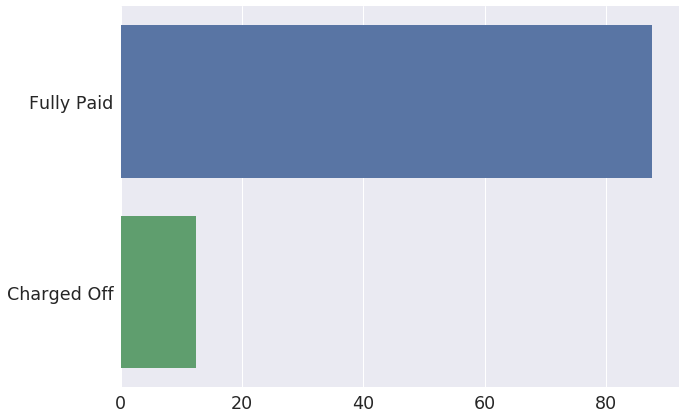
loan_status
Categorical
| Distinct count | 2 |
|---|---|
| Unique (%) | 0.0% |
| Missing (%) | 0.0% |
| Missing (n) | 0 |
| Fully Paid | |
|---|---|
| Charged Off | 21392 |
| Value | Count | Frequency (%) | |
| Fully Paid | 151353 | 87.6% | |
| Charged Off | 21392 | 12.4% |
percent_bc_gt_75
Numeric
| Distinct count | 135 |
|---|---|
| Unique (%) | 0.1% |
| Missing (%) | 21.0% |
| Missing (n) | 36346 |
| Infinite (%) | 0.0% |
| Infinite (n) | 0 |
| Mean | 52.646 |
|---|---|
| Minimum | 0 |
| Maximum | 100 |
| Zeros (%) | 12.5% |

Quantile statistics
| Minimum | 0 |
|---|---|
| 5-th percentile | 0 |
| Q1 | 25 |
| Median | 50 |
| Q3 | 80 |
| 95-th percentile | 100 |
| Maximum | 100 |
| Range | 100 |
| Interquartile range | 55 |
Descriptive statistics
| Standard deviation | 34.436 |
|---|---|
| Coef of variation | 0.6541 |
| Kurtosis | -1.2091 |
| Mean | 52.646 |
| MAD | 29.443 |
| Skewness | -0.08618 |
| Sum | 7180800 |
| Variance | 1185.8 |
| Memory size | 1.3 MiB |

| Value | Count | Frequency (%) | |
| 100.0 | 28569 | 16.5% | |
| 0.0 | 21592 | 12.5% | |
| 50.0 | 16685 | 9.7% | |
| 66.7 | 11432 | 6.6% | |
| 33.3 | 9277 | 5.4% | |
| 75.0 | 7375 | 4.3% | |
| 25.0 | 5676 | 3.3% | |
| 60.0 | 4310 | 2.5% | |
| 40.0 | 4208 | 2.4% | |
| 80.0 | 4152 | 2.4% | |
| Other values (124) | 23123 | 13.4% | |
| (Missing) | 36346 | 21.0% |
Minimum 5 values
| Value | Count | Frequency (%) | |
| 0.0 | 21592 | 12.5% | |
| 0.2 | 3 | 0.0% | |
| 0.25 | 2 | 0.0% | |
| 0.29 | 1 | 0.0% | |
| 0.33 | 17 | 0.0% |
Maximum 5 values
| Value | Count | Frequency (%) | |
| 93.3 | 3 | 0.0% | |
| 93.7 | 3 | 0.0% | |
| 94.1 | 2 | 0.0% | |
| 94.4 | 1 | 0.0% | |
| 100.0 | 28569 | 16.5% |
purpose
Categorical
| Distinct count | 14 |
|---|---|
| Unique (%) | 0.0% |
| Missing (%) | 0.0% |
| Missing (n) | 0 |
| debt_consolidation | |
|---|---|
| credit_card | |
| other | 10214 |
| Other values (11) |
| Value | Count | Frequency (%) | |
| debt_consolidation | 94874 | 54.9% | |
| credit_card | 39270 | 22.7% | |
| other | 10214 | 5.9% | |
| home_improvement | 9817 | 5.7% | |
| major_purchase | 4690 | 2.7% | |
| small_business | 3342 | 1.9% | |
| car | 2616 | 1.5% | |
| wedding | 1892 | 1.1% | |
| medical | 1877 | 1.1% | |
| moving | 1427 | 0.8% | |
| Other values (4) | 2726 | 1.6% |
revol_util
Numeric
| Distinct count | 1063 |
|---|---|
| Unique (%) | 0.6% |
| Missing (%) | 0.1% |
| Missing (n) | 144 |
| Infinite (%) | 0.0% |
| Infinite (n) | 0 |
| Mean | 55.829 |
|---|---|
| Minimum | 0 |
| Maximum | 140.4 |
| Zeros (%) | 0.7% |

Quantile statistics
| Minimum | 0 |
|---|---|
| 5-th percentile | 11 |
| Q1 | 38.6 |
| Median | 57.9 |
| Q3 | 75.1 |
| 95-th percentile | 92.2 |
| Maximum | 140.4 |
| Range | 140.4 |
| Interquartile range | 36.5 |
Descriptive statistics
| Standard deviation | 24.413 |
|---|---|
| Coef of variation | 0.43729 |
| Kurtosis | -0.68504 |
| Mean | 55.829 |
| MAD | 20.246 |
| Skewness | -0.32716 |
| Sum | 9636100 |
| Variance | 596.01 |
| Memory size | 1.3 MiB |

| Value | Count | Frequency (%) | |
| 0.0 | 1265 | 0.7% | |
| 64.6 | 301 | 0.2% | |
| 61.5 | 296 | 0.2% | |
| 66.5 | 293 | 0.2% | |
| 63.0 | 291 | 0.2% | |
| 61.3 | 289 | 0.2% | |
| 58.3 | 287 | 0.2% | |
| 66.6 | 282 | 0.2% | |
| 55.9 | 281 | 0.2% | |
| 62.6 | 280 | 0.2% | |
| Other values (1052) | 168736 | 97.7% |
Minimum 5 values
| Value | Count | Frequency (%) | |
| 0.0 | 1265 | 0.7% | |
| 0.1 | 118 | 0.1% | |
| 0.2 | 103 | 0.1% | |
| 0.3 | 89 | 0.1% | |
| 0.4 | 76 | 0.0% |
Maximum 5 values
| Value | Count | Frequency (%) | |
| 120.2 | 2 | 0.0% | |
| 122.5 | 1 | 0.0% | |
| 127.6 | 1 | 0.0% | |
| 128.1 | 1 | 0.0% | |
| 140.4 | 1 | 0.0% |
Sample
Predictive Modeling
def to_xy(dataset):
    y = dataset.pop('loan_status').cat.codes
    X = pd.get_dummies(dataset, drop_first=True)
    return X, y
Initializing Train/Test Sets
Shuffle and Split Data
Let’s split the data (both features and their labels) into training and test sets. 80% of the data will be used for training and 20% for testing.
Run the code cell below to perform this split.
X, y = load_and_preprocess_data().pipe(to_xy)

split_data = train_test_split(X, y, test_size=0.20, stratify=y, random_state=11)
X_train, X_test, y_train, y_test = split_data

train_test_sets = dict(
    zip(['X_train', 'X_test', 'y_train', 'y_test'], [*split_data]))
(pd.DataFrame(
    data={'Observations (#)': [X_train.shape[0], X_test.shape[0]],
          'Percent (%)': ['80%', '20%'],
          'Features (#)': [X_train.shape[1], X_test.shape[1]]},
    index=['Training', 'Test'])
 [['Percent (%)', 'Features (#)', 'Observations (#)']])
| Percent (%) | Features (#) | Observations (#) | |
|---|---|---|---|
| Training | 80% | 34 | 138196 |
| Test | 20% | 34 | 34549 |
Classification Models
Naive Predictor (Baseline)
dummy_model = LearningModel(
    'Naive Predictor - Baseline', Pipeline([
        ('imp', Imputer(strategy='median')),
        ('clf', DummyClassifier(strategy='constant', constant=0))]))

dummy_model.fit_and_predict(**train_test_sets)

model_evals = eval_db(dummy_model.eval_report)
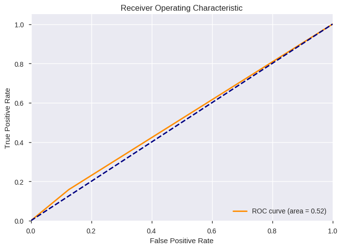
Decision Tree Classifier
tree_model = LearningModel(
    'Decision Tree Classifier', Pipeline([
        ('imp', Imputer(strategy='median')),
        ('clf', DecisionTreeClassifier(class_weight='balanced', random_state=11))]))

tree_model.fit_and_predict(**train_test_sets)
tree_model.display_evaluation()

model_evals = eval_db(model_evals, tree_model.eval_report)
| FitTime | Accuracy | FBeta | F1 | AUC | |
|---|---|---|---|---|---|
| Decision Tree Classifier | 2.0 | 0.78558 | 0.156742 | 0.154531 | 0.516244 |
             precision    recall  f1-score   support

          0       0.88      0.87      0.88     30271
          1       0.15      0.16      0.15      4278

avg / total       0.79      0.79      0.79     34549
Random Forest Classifier
rf_model = LearningModel(
    'Random Forest Classifier', Pipeline([
        ('imp', Imputer(strategy='median')),
        ('clf', RandomForestClassifier(
            class_weight='balanced_subsample', random_state=11))]))

rf_model.fit_and_predict(**train_test_sets)
rf_model.display_evaluation()

model_evals = eval_db(model_evals, rf_model.eval_report)
| FitTime | Accuracy | FBeta | F1 | AUC | |
|---|---|---|---|---|---|
| Random Forest Classifier | 2.0 | 0.874671 | 0.008998 | 0.014117 | 0.573608 |
             precision    recall  f1-score   support

          0       0.88      1.00      0.93     30271
          1       0.27      0.01      0.01      4278

avg / total       0.80      0.87      0.82     34549
Blagging Classifier
Base Estimator -> RF
blagging_pipeline = Pipeline([
    ('imp', Imputer(strategy='median')),
    ('clf', BlaggingClassifier(
        random_state=11, n_jobs=-1,
        base_estimator=RandomForestClassifier(
            class_weight='balanced_subsample', random_state=11)))])

blagging_model = LearningModel('Blagging Classifier (RF)', blagging_pipeline)

blagging_model.fit_and_predict(**train_test_sets)
blagging_model.display_evaluation()

model_evals = eval_db(model_evals, blagging_model.eval_report)
| FitTime | Accuracy | FBeta | F1 | AUC | |
|---|---|---|---|---|---|
| Blagging Classifier (RF) | 2.0 | 0.719181 | 0.344518 | 0.270746 | 0.645877 |
             precision    recall  f1-score   support

          0       0.90      0.76      0.83     30271
          1       0.20      0.42      0.27      4278

avg / total       0.82      0.72      0.76     34549
Base Estimator -> ExtraTrees
blagging_clf = BlaggingClassifier(
    random_state=11, n_jobs=-1,
    base_estimator=ExtraTreesClassifier(
        criterion='entropy', class_weight='balanced_subsample',
        max_features=None, n_estimators=60, random_state=11))

blagging_model = LearningModel(
    'Blagging Classifier (Extra Trees)', Pipeline([
        ('imp', Imputer(strategy='median')),
        ('clf', blagging_clf)]))

blagging_model.fit_and_predict(**train_test_sets)
blagging_model.display_evaluation()

model_evals = eval_db(model_evals, blagging_model.eval_report)
| FitTime | Accuracy | FBeta | F1 | AUC | |
|---|---|---|---|---|---|
| Blagging Classifier (Extra Trees) | 19.0 | 0.749718 | 0.309224 | 0.259611 | 0.645899 |
             precision    recall  f1-score   support

          0       0.90      0.81      0.85     30271
          1       0.20      0.35      0.26      4278

avg / total       0.81      0.75      0.78     34549
Evaluating Model Performance
Feature Importance (via RandomForestClassifier)
rf_top_features = LearningModel('Random Forest Classifier',
    Pipeline([('imp', Imputer(strategy='median')),
              ('clf', RandomForestClassifier(max_features=None,
                  class_weight='balanced_subsample', random_state=11))]))

rf_top_features.fit_and_predict(**train_test_sets)
rf_top_features.display_top_features(top_n=15)
| Feature | Score | |
|---|---|---|
| 1 | dti | 0.115602 |
| 2 | earliest_cr_line_age | 0.115381 |
| 3 | revol_util | 0.109714 |
| 4 | annual_inc | 0.099535 |
| 5 | loan_amnt | 0.080153 |
| 6 | bc_util | 0.077465 |
| 7 | fico_range_low | 0.071342 |
| 8 | avg_cur_bal_to_loan_amnt | 0.062594 |
| 9 | avg_cur_bal_to_inc | 0.052817 |
| 10 | avg_cur_bal | 0.050275 |
| 11 | emp_length | 0.047003 |
| 12 | percent_bc_gt_75 | 0.034591 |
| 13 | home_ownership_RENT | 0.009037 |
| 14 | purpose_credit_card | 0.008536 |
| 15 | purpose_debt_consolidation | 0.007986 |
rf_top_features.plot_top_features(top_n=10)
Model Selection
Comparative Analysis
display(model_evals)
| FitTime | Accuracy | FBeta | F1 | AUC | |
|---|---|---|---|---|---|
| Naive Predictor - Baseline | 0.0 | 0.876176 | 0.000000 | 0.000000 | 0.500000 |
| Decision Tree Classifier | 2.0 | 0.785580 | 0.156742 | 0.154531 | 0.516244 |
| Random Forest Classifier | 2.0 | 0.874671 | 0.008998 | 0.014117 | 0.573608 |
| Blagging Classifier (RF) | 2.0 | 0.719181 | 0.344518 | 0.270746 | 0.645877 |
| Blagging Classifier (Extra Trees) | 19.0 | 0.749718 | 0.309224 | 0.259611 | 0.645899 |
Optimal Model
blagging_model = LearningModel('Blagging Classifier (Extra Trees)',
    Pipeline([('imp', Imputer(strategy='median')),
              ('clf', BlaggingClassifier(
                  base_estimator=ExtraTreesClassifier(
                      criterion='entropy', class_weight='balanced_subsample',
                      max_features=None, n_estimators=60, random_state=11),
                  random_state=11, n_jobs=-1))]))

blagging_model.fit_and_predict(**train_test_sets)
Optimizing Hyperparameters
ToDo: Perform GridSearch…
Results:
(pd.DataFrame(data={'Benchmark Predictor': [0.7899, 0.1603, 0.5203],
                   'Unoptimized Model': [0.7499, 0.2602, 0.6463],
                   'Optimized Model': ['', '', '']},
             index=['Accuracy Score', 'F1-score', 'AUC'])
 [['Benchmark Predictor', 'Unoptimized Model', 'Optimized Model']])
| Benchmark Predictor | Unoptimized Model | Optimized Model | |
|---|---|---|---|
| Accuracy Score | 0.7899 | 0.7499 | |
| F1-score | 0.1603 | 0.2602 | |
| AUC | 0.5203 | 0.6463 |